SRW Example #1 (kick matrix)

Problem

Calculating electron trajectory in 3D magnetic field of an APPLE-II undulator, from the tabulated field and from a kick-matrix

Example Solution

• 
• 
• 
• 

Out:

SRWLIB Python Example # 1:
Calculating electron trajectory in 3D magnetic field of an APPLE-II undulator, from the tabulated field and from a kick-matrix
   Reading magnetic field data from files ... done
   Performing calculation ... done
   Plotting the results (close all graph windows to proceed with the script execution) ... done

from __future__ import print_function #Python 2.7 compatibility
from srwpy.srwlib import *
from srwpy.uti_plot import *
import os

print('SRWLIB Python Example # 1:')
print('Calculating electron trajectory in 3D magnetic field of an APPLE-II undulator, from the tabulated field and from a kick-matrix')

#**********************Input/Output File Names:
strExDataFolderName = 'data_example_01' #example data sub-folder name
arFldInFileNames = ['epu49HEtot.dat'] #3D Magnetic Field data file names
arKickMatrInFileNames = ['epu49he_kick_m.dat'] #Kick Matrix file names
strCenTrajOutFileName = 'ex01_res_traj.dat' #file name for output trajectory data
strOffTrajOutFileName = 'ex01_res_traj_off.dat' #file name for output trajectory data
strOffKickTrajOutFileName = 'ex01_res_traj_kick_off.dat' #file name for output trajectory data

#**********************Auxiliary function to read a matrix from a file:
def AuxReadInMatrix(f, nx, ny, nch):
    nx = int(round(nx)) #int() required for Python 2.7 compatibility
    ny = int(round(ny))
    nch = int(round(nch))
    flatM = [0]*ny*nx
    ic = 0
    for iy in range(ny):
        s = f.readline()
        pSep = 0
        pSepNext = nch
        for ix in range(nx):
            sCur = s[pSep:pSepNext]
            isNonNum = 1
            for i in range(nch):
                if sCur[i] != ' ':
                    isNonNum = 0
                    break
            if isNonNum == 0:
                flatM[ic] = float(sCur)
            else:
                flatM[ic] = 0
            pSep = pSepNext
            pSepNext += nch
            ic += 1
    return flatM

#**********************Auxiliary function to read tabulated Kick-Matrix data (Radia format):
def AuxReadInKickM(filePath, sCom):
    f = open(filePath, 'r')
    f.readline() #1st line: just pass
    f.readline() #2nd line: just pass
    f.readline() #3rd line: just pass
    rz = float(f.readline()) #4th line: longitudinal range
    f.readline() #5th line: just pass
    nx = int(f.readline()) #6th line: number of points in horizontal direction
    f.readline() #7th line: just pass
    ny = int(f.readline()) #8th line: number of points in vertical direction
    f.readline() #9th line: just pass
    f.readline() #10th line: just pass "START"
    flatKickMx = AuxReadInMatrix(f, nx + 1, ny + 1, 14)
    f.readline() #just pass
    f.readline() #just pass "START"
    flatKickMy = AuxReadInMatrix(f, nx + 1, ny + 1, 14)
    f.readline() #just pass
    f.readline() #just pass "START"
    #IntB2 = AuxReadInMatrix(f, nx + 1, ny + 1, 14)
    arMx = array('d', [0]*nx*ny)
    arMy = array('d', [0]*nx*ny)
    i = 0
    for iy in range(1, ny + 1):
        for ix in range(1, nx + 1):
            #arMx[i] = KickMx[ix][iy]
            #arMy[i] = KickMy[ix][iy]
            #print(ix, iy, i, arMx[i])
            ofst = (ny + 1 - iy)*(nx + 1) + ix
            arMx[i] = flatKickMx[ofst]
            arMy[i] = flatKickMy[ofst]
            #print(ix, iy, i, arMx[i])
            i += 1
    #xMin = KickMx[1][0]
    #xMax = KickMx[nx][0]
    xMin = flatKickMx[1]
    xMax = flatKickMx[nx]
    xc = 0.5*(xMin + xMax)
    rx = xMax - xMin
    #yMin = KickMx[0][1]
    #yMax = KickMx[0][ny]
    yMax = flatKickMx[1*(nx + 1)]
    yMin = flatKickMx[ny*(nx + 1)]
    yc = 0.5*(yMin + yMax)
    ry = yMax - yMin
    return SRWLKickM(arMx, arMy, 2, nx, ny, 1, rx, ry, rz, xc, yc, 0)

#**********************Auxiliary function to read tabulated 3D Magnetic Field data from ASCII file:
def AuxReadInMagFld3D(filePath, sCom):
    f = open(filePath, 'r')
    f.readline() #1st line: just pass
    xStart = float(f.readline().split(sCom, 2)[1]) #2nd line: initial X position [m]; it will not actually be used
    xStep = float(f.readline().split(sCom, 2)[1]) #3rd line: step vs X [m]
    xNp = int(f.readline().split(sCom, 2)[1]) #4th line: number of points vs X
    yStart = float(f.readline().split(sCom, 2)[1]) #5th line: initial Y position [m]; it will not actually be used
    yStep = float(f.readline().split(sCom, 2)[1]) #6th line: step vs Y [m]
    yNp = int(f.readline().split(sCom, 2)[1]) #7th line: number of points vs Y
    zStart = float(f.readline().split(sCom, 2)[1]) #8th line: initial Z position [m]; it will not actually be used
    zStep = float(f.readline().split(sCom, 2)[1]) #9th line: step vs Z [m]
    zNp = int(f.readline().split(sCom, 2)[1]) #10th line: number of points vs Z
    totNp = xNp*yNp*zNp
    locArBx = array('d', [0]*totNp)
    locArBy = array('d', [0]*totNp)
    locArBz = array('d', [0]*totNp)
    for i in range(totNp):
        curLineParts = f.readline().split('\t')
        locArBx[i] = float(curLineParts[0])
        locArBy[i] = float(curLineParts[1])
        locArBz[i] = float(curLineParts[2])
    f.close()
    xRange = xStep
    if xNp > 1: xRange = (xNp - 1)*xStep
    yRange = yStep
    if yNp > 1: yRange = (yNp - 1)*yStep
    zRange = zStep
    if zNp > 1: zRange = (zNp - 1)*zStep
    return SRWLMagFld3D(locArBx, locArBy, locArBz, xNp, yNp, zNp, xStep*(xNp - 1), yStep*(yNp - 1), zStep*(zNp - 1), 1)

#**********************Input Parameters and Input/Output structures:
partTraj = SRWLPrtTrj() #Central Trajectory
partTraj.partInitCond.x = 0 #Initial Transverse Coordinates (initial Longitudinal Coordinate will be defined later on) [m]
partTraj.partInitCond.y = 0
newInitCondX = 0.004 #Initial Transverse Coordinates for Off-Axis Trajectory [m]
newInitCondY = 0.0005
partTraj.partInitCond.xp = 0 #Initial Transverse Velocities
partTraj.partInitCond.xp = 0
partTraj.partInitCond.gamma = 3/0.51099890221e-03 #Relative Energy
partTraj.partInitCond.relE0 = 1 #Electron Rest Mass
partTraj.partInitCond.nq = -1 #Electron Charge

partTraj.ctStart = 0 #Start Time for the calculation
partTraj.ctEnd = 2.5 #magFldCnt.arMagFld[0].rz
partTraj.allocate(10001) #Number of Points for Trajectory calculation

arPrecTrajFromField = [1] #Precision parameters for Trajectory calculation from Field:
#[0]: integration method No:
    #1- fourth-order Runge-Kutta (precision is driven by number of points)
    #2- fifth-order Runge-Kutta
#[1],[2],[3],[4],[5]: absolute precision values for X[m],X'[rad],Y[m],Y'[rad],Z[m] (yet to be tested!!) - to be taken into account only for R-K fifth order or higher
#[6]: tolerance (default = 1) for R-K fifth order or higher
#[7]: max. number of auto-steps for R-K fifth order or higher (default = 5000)

arPrecTrajFromKickM = [1] #Precision parameters for Trajectory calculation from Kick-Matrices:
#[0]: switch specifying whether the new trajectory data should be added to pre-existing trajectory data (=1, default)
#or it should override any pre-existing trajectory data (=0)

#**********************Defining Magnetic Field:
magFldCnt = SRWLMagFldC() #Container
magFldCnt.allocate(1) #Magnetic Field consists of 1 part
print('   Reading magnetic field data from files ... ', end='')
filePath = os.path.join(os.getcwd(), strExDataFolderName, arFldInFileNames[0])
magFldCnt.arMagFld[0] = AuxReadInMagFld3D(filePath, '#')
print('done')

magFldCnt.arXc[0] = 0 #Transverse Coordinates of ID Center [m]
magFldCnt.arYc[0] = 0
magFldCnt.arZc[0] = 0 #Longitudinal Coordinate of ID Center [m]

magFldCnt.arMagFld[0].interp = 3 #Magnetic Field Interpolation Method, to be entered into 3D field structures below (to be used e.g. for trajectory calculation):
#1- bi-linear (3D), 2- bi-quadratic (3D), 3- bi-cubic (3D), 4- 1D cubic spline (longitudinal) + 2D bi-cubic

magFldCnt.arMagFld[0].nRep = 1 #Number of parts of ID
partTraj.partInitCond.z = -0.5*magFldCnt.arMagFld[0].rz #Initial Longitudinal Coordinate (before ID)

#**********************Defining Kick Matrices:
filePath = os.path.join(os.getcwd(), strExDataFolderName, arKickMatrInFileNames[0])
kickMatr = AuxReadInKickM(filePath, '#')

#**********************Calculation (SRWLIB function call)
print('   Performing calculation ... ', end='')

srwl.CalcPartTraj(partTraj, magFldCnt, arPrecTrajFromField) #First Calculate Central Trajectory
partTraj.save_ascii(os.path.join(os.getcwd(), strExDataFolderName, strCenTrajOutFileName))

partTraj.partInitCond.x = newInitCondX
partTraj.partInitCond.y = newInitCondY
srwl.CalcPartTrajFromKickMatr(partTraj, kickMatr, arPrecTrajFromKickM)#Calculate Off-Axis Trajectory using Kick-Matrix method
partTraj.save_ascii(os.path.join(os.getcwd(), strExDataFolderName, strOffKickTrajOutFileName))

srwl.CalcPartTraj(partTraj, magFldCnt, arPrecTrajFromField) #Calculate same Off-Axis Trajectory by Runge-Kutta integration in 3D Magnetic Field
partTraj.save_ascii(os.path.join(os.getcwd(), strExDataFolderName, strOffTrajOutFileName))

print('done')

#**********************Plotting results
print('   Plotting the results (close all graph windows to proceed with the script execution) ... ', end='')
ctMesh = [partTraj.ctStart, partTraj.ctEnd, partTraj.np]
for i in range(partTraj.np): #converting from [m] to [mm] and from [rad] to [mrad]
    partTraj.arX[i] *= 1000
    partTraj.arXp[i] *= 1000
    partTraj.arY[i] *= 1000
    partTraj.arYp[i] *= 1000

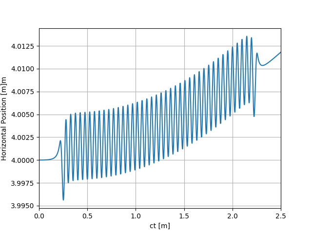
uti_plot1d(partTraj.arX, ctMesh, ['ct [m]', 'Horizontal Position [m]m'])
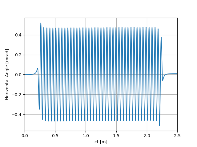
uti_plot1d(partTraj.arXp, ctMesh, ['ct [m]', 'Horizontal Angle [mrad]'])
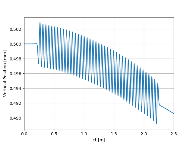
uti_plot1d(partTraj.arY, ctMesh, ['ct [m]', 'Vertical Position [mm]'])
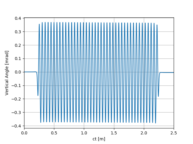
uti_plot1d(partTraj.arYp, ctMesh, ['ct [m]', 'Vertical Angle [mrad]'])
uti_plot_show()
print('done')